Application 1: forecast from the 2022Q2 inflation peak¶

This is the main tutorial. It takes one question through the whole toolbox: the scenario files, the run, what happens inside it, the output files, and the results with the figures and numbers of the project's baseline (summary tables in results/summary_v3/).

The question. US inflation (GDP deflator) peaked in 2022Q2 at 8.9% annualized. Suppose that from that quarter on no further shocks hit the economy. How fast does inflation come down if every agent has rational expectations (RE), and how fast if part of the population forms inflation expectations by adaptive learning, with the share of learners moving with recent forecast performance?

Result in one line

With learners, average inflation over 2022Q3-2026Q2 is 3.45% against 2.59% under rational expectations. The gap peaks at +3.54 percentage points (pp) in 2023Q1. The learners' share of inflation expectations is 0.591 at the origin and rises to 0.685 in 2023Q1, because the learners' perceived persistence of inflation is above one at the peak (AR(1) coefficient 1.061).

1. The model and the data¶

The model package is models/sw07/: the Smets and Wouters (2007) model (SW07), log-linear, seven shocks, seven US observables (output, consumption and investment growth, real wage growth, hours, inflation, the federal funds rate). The project baseline uses the published SW07 posterior mode for 1966Q1-2004Q4 (models/sw07/sw07_params_original.m). The database runs from 1965Q1 to 2026Q2 (FRED vintage 2026-09-29); every observable is treated as missing in the COVID-19 quarters (2020Q1-2020Q3), so the Kalman filter skips them.

SW07 has twelve forward-looking variables. In Application 1 only inflation, pinf, has heterogeneous expectations; every other expectation stays rational.

2. Expectations in the learning economy¶

In the learning economy every one-step expectation of inflation is a weighted average of two forecasts, the RE agents' and the learners', with weights equal to the population shares. The shares in force in quarter t are those computed at the end of t-1 (Expectations, Timing and information).

RE agents are anchored and see data up to t-1. Their forecast is that of the pure-RE model in which inflation expectations are formed with data up to t-1, evaluated at the current state (RE agents).

Learners believe inflation follows an AR(1) with a constant, their perceived law of motion (PLM). They also see data up to t-1, so they iterate the PLM two steps ahead (Perceived laws of motion). After inflation in t is observed they update the two coefficients by recursive least squares (Gains). The code's suffix for the learners is BR, for bounded rationality.

The gain of that update is endogenous (Kostyshyna, Özden and Zhang 2024, eq. 9). It starts at 0.05, rises when the learners' errors keep the same sign, falls when they alternate, and stays inside [0.001, 0.25] (Gains).

Shares follow the discrete choice of Özden (2025, eqs. 14-15). Each type's fitness is a discounted sum of its past squared forecast errors, in percent per quarter, with memory 0.8; the learners' share is a logit in the two fitness values with intensity of choice 2 (Shares and switching).

Stability. Each quarter the model with the new beliefs and shares, the actual law of motion (ALM), is solved. If it has no stable solution, the projection facility puts the beliefs back to their values before the update (projection.facility = 'alm'; Projection facility). In Application 1 this never happens.

3. The baseline settings¶

The settings above are the project baseline, set once in config/master_options.m so that every scenario of the project inherits them:

% config/master_options.m (excerpt)
o.model_params = 'sw07_params_original';   % published SW07 (2007) mode
o.gain.rule = 'koz';                       % endogenous gain, Kostyshyna, Ozden and Zhang (2024)
o.gain.value = 0.05;                       % start gain
o.switching.intensity = 2;                 % chi
o.switching.memory = 0.8;                  % omega
o.shares.init_n2 = 0.5;                    % initial share of learners
o.beliefs.plm.default = 'ar1';             % AR(1) PLM with constant
o.beliefs.info = 'lagged';                 % learners see data up to t-1
o.expectations.re_info = 'lagged';         % RE agents: E_{t-1} x_{t+1}
o.expectations.re_variant = 'anchored';    % RE agents use the pure-RE forecast
o.history.re_states = 'filtered';          % history from the one-sided RE filter
o.projection.facility = 'alm';             % facility on the actual law of motion

These values differ from the toolbox defaults in hetlearn.defaults() (constant gain 0.0585, intensity of choice 0.51, memory 0.6, period-t RE information, smoothed history, facility 'plm_alm'). A new project starts from the defaults and sets its own baseline in its config/master_options.m.

4. The scenario files¶

Every SW07 scenario descends from one parent, scenarios/sw07/base/sw07_re.m. It sets the model, finds the inflation peak and fixes the horizon. It also lists every other option as a commented line, so it doubles as a template:

function cfg = sw07_re()
cfg = struct();
cfg.id = 'sw07_re';
cfg.title = 'Forecast from the 2022Q2 inflation peak, rational expectations';
cfg.model = 'sw07';                           % model package models/sw07/

% forecast origin: the quarter of peak inflation in 2020Q1-2024Q4
spec = hetlearn.load_spec(cfg.model);
db = hetlearn.load_database(spec);
origin = hetlearn.find_peak(db, 'pinfobs', qq(2020, 1), qq(2024, 4));
assert(hetlearn.util.date_eq(origin, qq(2022, 2)), ...
    'sw07_re: expected the inflation peak in 2022Q2, found %s.', char(dat2str(origin)));
cfg.forecast.origin = origin;                 % last quarter of data used
cfg.forecast.horizon = 16;                    % quarters: 2022Q3-2026Q2

cfg.expectations.mode = 'rational';           % every agent RE
cfg.expectations.variables = {'pinf'};        % inflation has the RE/BR block
% ... every other option, commented, at its inherited value
end

In mode 'rational' the inflation block is in the model with an RE share of 1, so the run is the RE model (with t-1 information for inflation, from the baseline). Beliefs and shares are still tracked as diagnostics.

The learning parent switches the shares on:

function cfg = sw07_learn()
cfg = sw07_re();
cfg.id = 'sw07_learn';
cfg.expectations.mode = 'switching';
cfg.compare_with = {'sw07_re'};
end

Application 1 is these two scenarios under their own names (scenarios/sw07/app1_peak/):

function cfg = a1_re()
cfg = sw07_re();
cfg.id = 'a1_re';
cfg.title = 'App 1: forecast from the 2022Q2 peak, rational expectations';
end

function cfg = a1_learn()
cfg = sw07_learn();
cfg.id = 'a1_learn';
cfg.title = 'App 1: forecast from the 2022Q2 peak, learning on inflation';
cfg.compare_with = {'a1_re'};                 % writes compare_a1_re.csv
end

a1_learn is the parent of every learning scenario in the other applications and the model variants, so a change here reaches all of them.

5. Run¶

setup_paths
run_applications('app1')         % a1_re, then a1_learn; one row each in results/run_log.csv

or, without the runner:

res_re = hetlearn.run(a1_re());
res    = hetlearn.run(a1_learn());

A failing run under run_applications is printed and logged, and the next one runs.

6. What happens inside a run¶

hetlearn.run(cfg) goes through these stages:

Stage	Function	What it does in Application 1
Options	`hetlearn.load_options`	Merges the defaults, `config/master_options.m` and `cfg` (order), checks every name and value
Package	`hetlearn.load_spec`	Reads `models/sw07/model_spec.m`
Model	`hetlearn.load_model`	Writes the extended model `models/sw07/generated/sw07_ext_ar1_relag.model` (once): every `pinf{+1}` becomes the mixed expectation of section 2. Checks that with RE shares of 1 it reproduces the original model (collapse test), computes the anchored-RE coefficients, solves
RE filter	`hetlearn.re_filter`	Kalman filter and smoother of the RE model over 1965Q1-2026Q2, cached in `generated/refilter_*.mat`
History	`hetlearn.engine.history`	Initial beliefs at 1966Q1 from the RE model's moments, initial share 0.5. Each quarter to 2022Q2: RE forecast and the learners' data from the one-sided RE filter, forecast errors, fitness and shares, the gain, the recursive least-squares update, the ALM check
Forecast	`hetlearn.engine.forecast`	From the smoothed 2022Q2 state, 16 quarters with zero shocks. Each quarter: the model with the current beliefs and shares is solved and simulated one quarter, then beliefs, gain and shares update on the simulated outcome
Save	`hetlearn.engine.save_results`	Writes `results/a1_learn/`

The engine asserts each quarter that the learners' forecast inside the model equals their PLM forecast with the beliefs of the end of t-1 on their information set.

7. The outputs¶

results/a1_learn/ holds:

File	Content
`results.mat`	`res`: `.cfg` (merged options), `.paths` (every variable and shock, 1965Q1-2026Q2: RE-smoothed history, then the forecast), `.learning`, `.events`, `.state`, `.dates`, `.meta`, `.loss`
`observables.csv`	The seven observables, history and forecast, model units
`paths.csv`	Every transition variable over the forecast horizon
`learning.csv`	Long format: date, variable, field, value
`events.csv`	Projection-facility and other events (empty for this run)
`compare_a1_re.csv`	Observables of `a1_learn` minus `a1_re` over the horizon
`loss.csv`	Discounted policy loss with the default weights (SW07 has a policy section)

The learning fields of res.learning.pinf: alpha_pinf, beta_pinf (beliefs), R_alpha_pinf, R_beta_pinf (diagonal of the moment matrix), gain, gain_R, n1, n2 (shares computed at the end of each quarter), n1_model (RE share in force in the model), zetaRE, zetaBR (fitness), FE_RE, FE_BR (squared errors), fRE, fBR (forecasts).

L = res.learning.pinf;
L.beta_pinf(qq(2022, 2))     % 1.0608
L.alpha_pinf(qq(2022, 2))    % 0.0827
L.gain(qq(2022, 2))          % 0.0499
L.n2(qq(2022, 2))            % 0.5907
res.events                   % empty table: the facility never acted

8. Results¶

Application 1

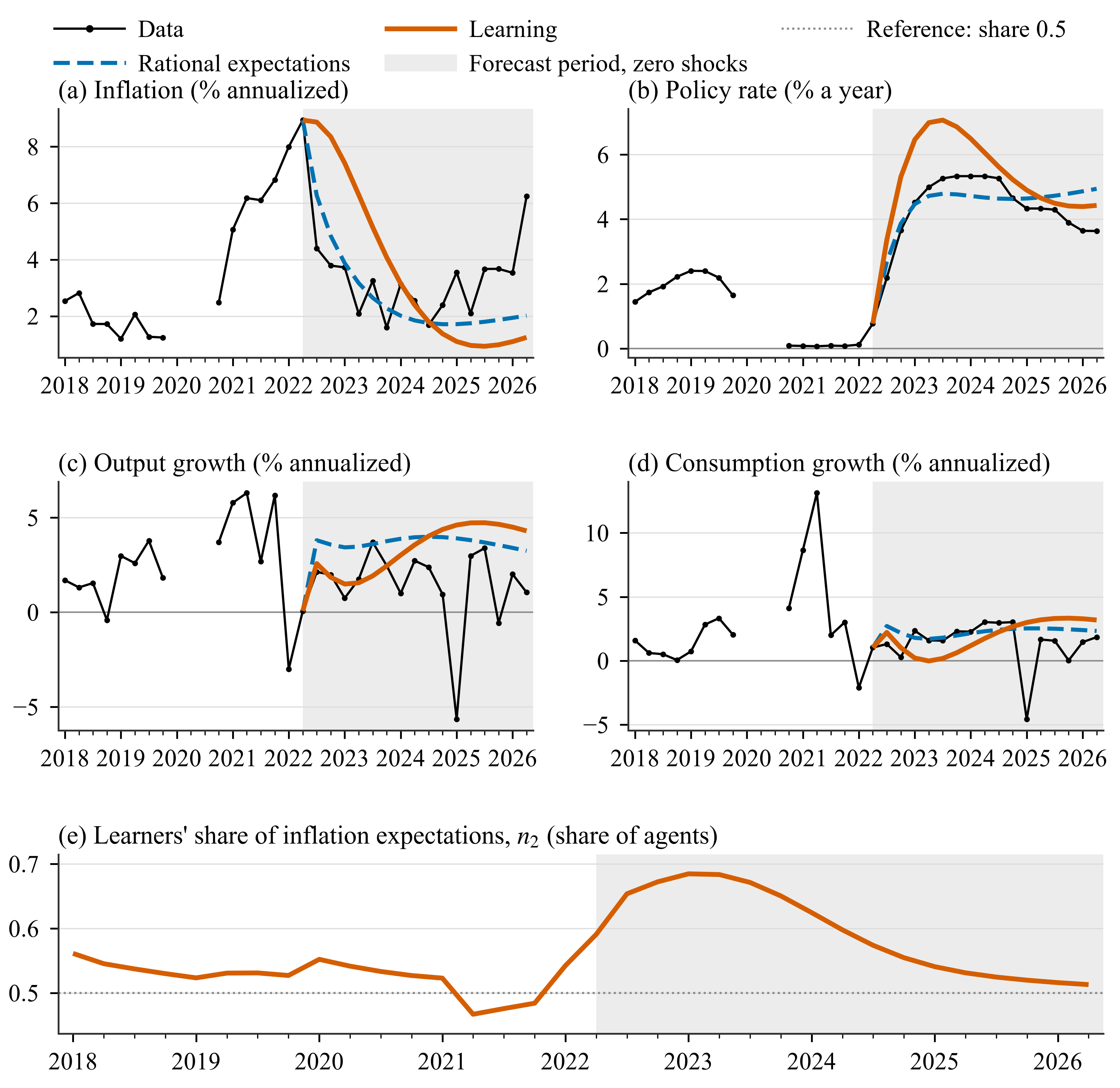
Panels a-d: data (black), RE benchmark a1_re (blue, dashed) and learning economy a1_learn (orange), annualized, with the forecast shaded. Panel e: the learners' end-of-quarter share \(n_2\). The data line has a gap in the 2020 quarters, treated as missing.

Averages of the forecast, in percent (inflation and growth rates quarter on quarter (q/q), annualized; policy rate % a year):

Variable	Data	RE	Learning	L − RE	Data	RE	Learning	L − RE
	2022Q3-2023Q2				2022Q3-2026Q2
Inflation	3.50	4.54	7.73	+3.20	3.21	2.59	3.45	+0.86
Policy rate	3.84	3.93	5.53	+1.59	4.41	4.53	5.42	+0.88
Output growth	1.65	3.57	1.86	−1.70	1.44	3.69	3.39	−0.29
Consumption growth	1.38	2.10	0.86	−1.24	1.42	2.27	1.96	−0.31

Inflation quarter by quarter (annualized):

Quarter	RE	Learning	Learners' share in force
2022Q3	6.27	8.87	0.591
2023Q2	3.17	6.30	0.685
2024Q2	1.85	2.39	0.625
2026Q2	2.02	1.25	0.516

Learners slow the disinflation. Under RE inflation falls from 8.9% to 6.3% in the first quarter and to 3.2% a year later; with learners it is still 8.9% in 2022Q3 and 6.3% a year later. At the origin the learners' AR(1) coefficient is 1.061: after the 2021-22 surge they perceive inflation as explosive, so their forecast extrapolates the peak, and while inflation stays high their forecasts do well and their share rises to 0.685. The Taylor rule responds to the higher inflation. The policy rate averages 5.42% against 4.53% under RE and peaks near 7% in 2023, and output and consumption growth are lower in the first year.

From 2024Q4 inflation in the learning economy is below the RE path (1.25% against 2.02% in 2026Q2), and the share drifts back toward 0.5, as in any zero-shock forecast (Shares and switching). Realized inflation averaged 3.21%, between the two forecasts. The data fell much faster than the learners' AR(1) predicted: on the data, the learners' share fell to 0.229 in 2022Q4 (next section).

9. The learners over the history¶

The learners' beliefs and share at the origin are the product of learning over 1966Q1-2022Q2. a6_smooth_learn is a1_learn with the origin moved to 2026Q2, so it shows the same history continued on the data:

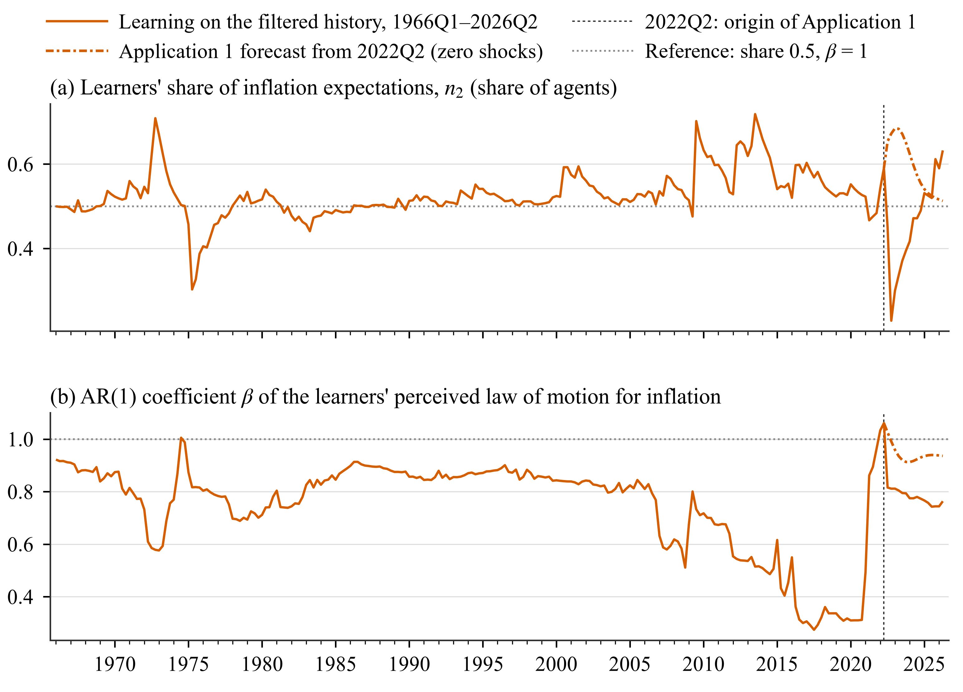
Learners' share and perceived persistence, 1966-2026

Panel a: the learners' end-of-quarter share \(n_2\). Panel b: the AR(1) coefficient \(\beta\) of their inflation PLM. Solid: learning on the RE-filtered history 1966Q1-2026Q2 (a6_smooth_learn); dash-dot: the Application 1 forecast from 2022Q2. The reference lines mark a share of 0.5 and \(\beta = 1\).

Statistic, 1966Q1-2022Q2	Share \(n_2\)	\(\beta\)
Mean	0.528	0.747
Minimum	0.303 (1975Q2)	0.274 (2017Q3)
Maximum	0.718 (2013Q3)	1.061 (2022Q2)

\(\beta\) is at or above 1 in three quarters only: 1974Q3, 2022Q1 and 2022Q2. The share was 0.527 at the end of 2019Q4, fell to 0.467 at the end of 2021Q2, when the first surge in inflation surprised the learners more than the RE agents, and rose to 0.591 at the end of 2022Q2.

10. Plotting from the result struct¶

The figures above are drawn from the summary tables. A new run can be plotted straight from res:

spec = hetlearn.load_spec('sw07');
db = hetlearn.load_database(spec);           % the data, with the 2020 gap
rng = qq(2018, 1):qq(2026, 2);

figure
subplot(2, 1, 1); hold on
plot(rng, 4*db.pinfobs, 'k.-')               % data
plot(rng, 4*res_re.paths.pinfobs, '--')      % RE benchmark
plot(rng, 4*res.paths.pinfobs)               % learning economy
title('Inflation, % q/q annualized'); legend('data', 'RE', 'learning')

subplot(2, 1, 2)
plot(rng, res.learning.pinf.n2)
title('Learners'' share, end of quarter')

11. Changing the assumptions¶

Each block below is a complete experiment; the last line compares them with a1_learn.

% Intensity of choice
cfg = a1_learn(); cfg.id = 'a1_chi051'; cfg.switching.intensity = 0.51;
hetlearn.run(cfg);

% Memory of the fitness measure
cfg = a1_learn(); cfg.id = 'a1_mem06'; cfg.switching.memory = 0.6;
hetlearn.run(cfg);

% Constant gain instead of the endogenous gain (model variant 4, v4_const)
cfg = a1_learn(); cfg.id = 'a1_const'; cfg.gain.rule = 'constant'; cfg.gain.value = 0.05;
hetlearn.run(cfg);

% Learners see period-t data (Ozden 2025, eq. 12)
cfg = a1_learn(); cfg.id = 'a1_info_t'; cfg.beliefs.info = 'current';
hetlearn.run(cfg);

% AR(2) learners (model variant 2, v2_ar2)
cfg = a1_learn(); cfg.id = 'a1_ar2'; cfg.beliefs.plm.default = 'ar2';
hetlearn.run(cfg);

T = hetlearn.compare({'a1_learn', 'a1_chi051', 'a1_mem06', 'a1_const', 'a1_info_t', 'a1_ar2'}, {'pinfobs'});

The project runs a set of such variants as saved scenarios. Average inflation over 2022Q3-2026Q2 and the learners' share at the end of 2022Q2:

Scenario	Change from `a1_learn`	Inflation (%)	Share at origin
`a1_re`	every agent rational	2.59
`a1_learn`	baseline	3.45	0.591
`v4_const`	`gain.rule = 'constant'`, `gain.value = 0.05`	3.50	0.595
`v4_decreasing`	`gain.rule = 'decreasing'`	3.12	0.618
`v5_chi050`	`switching.intensity = 0.5`	3.08	0.523
`v5_chi225`	`switching.intensity = 2.25`	3.74	0.602
`v5_omega075`	`switching.memory = 0.75`	3.88	0.610
`v5_omega095`	`switching.memory = 0.95`	3.19	0.559
`v2_ar2`	`beliefs.plm.default = 'ar2'`	3.69	0.599
`v2_ar1nc`	`beliefs.plm.default = 'ar1_noconst'`	3.25	0.611
`v2_reg`	inflation regressed on lagged inflation, output gap, rate	2.56	0.601
`v2_var3`	VAR(1) in inflation, output gap, rate	2.57	0.598
`v2_var12`	VAR(1) in the 12 forward-looking variables	3.19	0.611
`v1_mc_learn`	`expectations.re_variant = 'model_consistent'`	8.14	0.591
`v3_all`	`expectations.variables = 'all'` (facility `'alm'`)	14.50	0.698
`v3_all_plm_alm`	the same with facility `'plm_alm'`	2.72	0.694

The PLM matters most. The figure compares four of them:

Perceived laws of motion

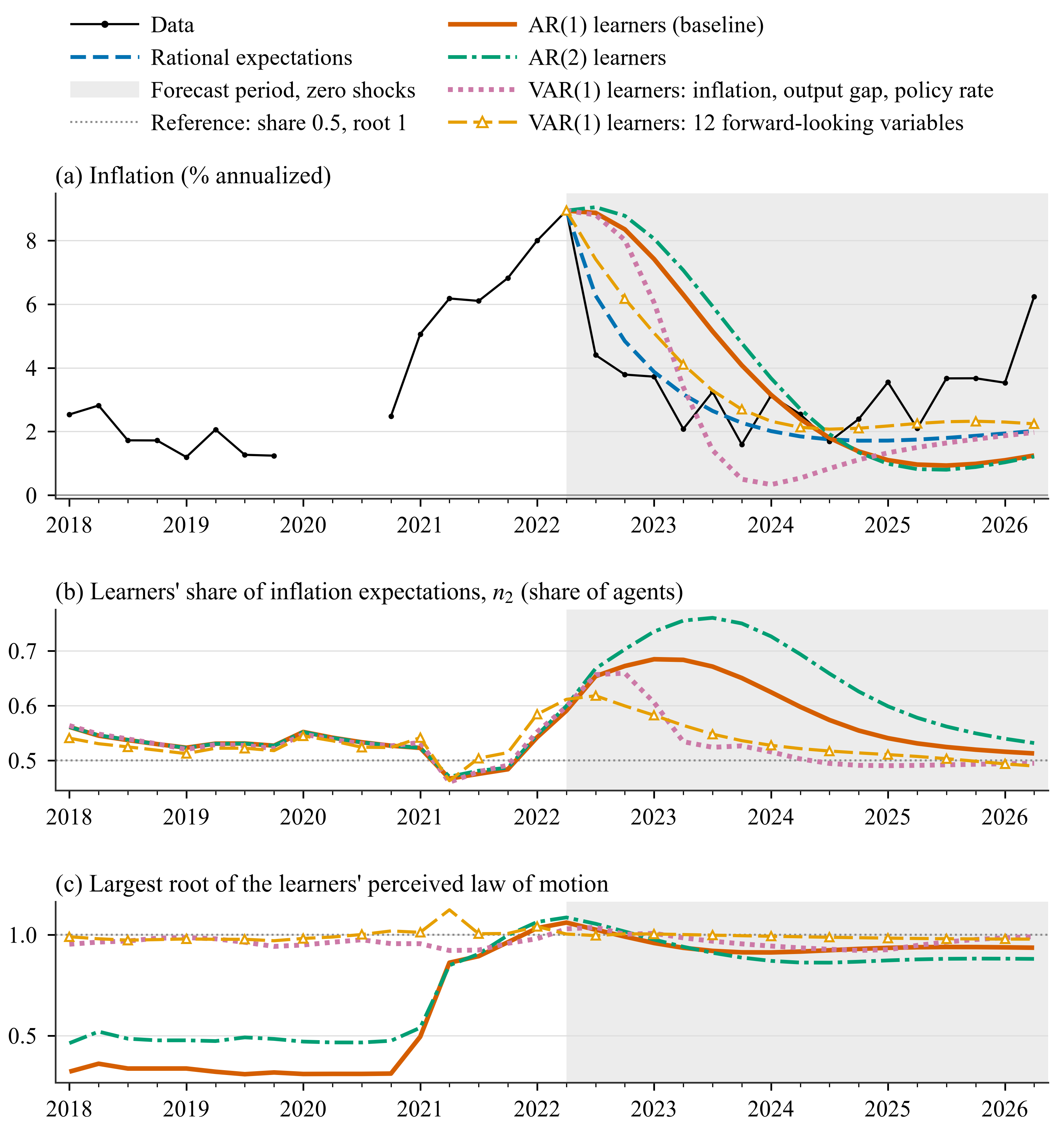
Inflation, the learners' share and the largest root of the PLM under the baseline AR(1), an AR(2) and two vector autoregressive (VAR(1)) PLMs; the reference line marks a root of 1. Every PLM has a largest root at or above 1 at the 2022Q2 origin (AR(1) 1.061, AR(2) 1.086, VAR(1) in three variables 1.030, VAR(1) in twelve variables 1.004).

Details for each option: Perceived laws of motion, Gains, Shares and switching, RE agents, Projection facility. The checks run on these results and the commands that reproduce them are on the Applications page.